COMPUTER VISION · PERSONAL HISTORICAL RECORD
Four terabytes.
A human responsibility.
Descriptors, classifiers, neural networks and the cost of searching for evidence with the resources of 2010–2011.
Klyff Harlley Toledo · November 2010 · Curitiba, Paraná
A personal account and scientific discussion of techniques. Quantitative figures are reproducible analytical scenarios, without data from the historical corpus.
Download the Python supplement ↓Contents · 22 sections
- 1. Before the first vector, there were people and hard drives
- 2. The laboratory that existed—and the future that did not yet exist
- 3. Preserve what arrived before interpreting what appears
- 4. From authorized observation to a byte stream
- 5. ZIP inside RAR inside another archive: the recursive problem
- 6. A separate network as an analysis environment
- 7. “It looks like an image” is still a format hypothesis
- 8. Four terabytes: research time sounded like an HDD
- 9. Fitting an image into a representation
- 10. Distance, normalization and what the number compares
- 11. Training a classifier did not mean writing a rule for every photograph
- 12. A dataset begins with human decisions
- 13. Content, age, identity and conclusions are different questions
- 14. CNNs: learned representations and an operation budget
- 15. Margins, probabilities and abstention
- 16. When 95% sensitivity still produces a poor queue
- 17. Human review is a finite resource
- 18. Personal record: 2012 and 2022
- 19. A verifiable procedure without disclosing the confidential implementation
- 20. What came later—a separate timeline
- 21. An analytical supplement to run at home
- 22. Conclusion: narrow the search and preserve uncertainty
Abstract
This article examines the computational and human challenges of organizing an image-triage pipeline to address child sexual exploitation, in the context of my master's studies in Curitiba between 2010 and 2011. The starting point is a corpus of approximately 4 TB received on hard drives through handover and accountability procedures involving Brazil's Federal Police, alongside the related problem of recovering objects from network streams under authorized observation. The method is divided into preservation, stream reassembly, format identification, controlled archive extraction, decoding, visual description, classification, calibration and human review. The discussion distinguishes local and global descriptors, statistical classifiers and convolutional networks available during that period; separates CPU processing, memory limits and storage costs; and explains why a score threshold does not establish age, authorship, identity or a forensic conclusion. Seven sets of reproducible figures and tables illustrate analytical costs and mathematical distributions. My photographs from 2012 and 2022 provide context for changes in appearance over ten years, without biometric comparison. The purpose is to document scientific techniques and decisions while protecting the corpus, the complete implementation, people under investigation and confidential information.
Keywords: computer vision; child protection; forensic triage; descriptors; CPU; SIFT; SURF; HOG; SVM; convolution; calibration; chain of custody.
1. Before the first vector, there were people and hard drives
I was an artificial-intelligence enthusiast pursuing a master's degree. Teaching a machine to perceive patterns was a fascinating idea. The problem that emerged, however, had none of the lightness of a laboratory demonstration: it involved images whose analysis could be necessary to protect children and support investigative work. Scientific motivation was inseparable from responsibility for the problem we were trying to address.
In my account of that work, the Federal Police handed over the material and there were documents to sign. The volume I remember was approximately 4 TB of photographs on HDDs: several heavy, slow drives containing previously organized images that needed to become working sets for classification. I do not publish the drive inventory, the provenance of individual files or the confidential documentation. The number conveys the physical scale of the challenge; it does not authorize redistribution of the content.
It took a strong stomach. But a professional response could not romanticize exposure or turn suffering into technical curiosity. I needed to reduce unnecessary viewing, control who accessed what and build a method that helped the people responsible for analysis, rather than simply multiplying the images they would have to see.
Two workstreams needed to communicate without being confused. One concerned the corpus received on physical media. The other concerned incoming and outgoing information streams associated with subjects whose observation was formally within the scope of an investigation. A file received on a drive does not have the same technical provenance as an object reassembled from traffic. A reliable report must preserve that distinction from the beginning.
The hard work began before artificial intelligence. I needed to establish what material had arrived, what had been copied, what was complete, what could not be decoded and what transformations had been performed for analysis. Only then did the visual question begin. And it was not a single question.
decodable image ≠ correctly interpreted content
high score ≠ established age ≠ forensic conclusion
This is the central argument of the article. A machine can help narrow a search, order a queue and expose uncertainty. It cannot turn a statistical indication into certainty merely because the software has finished running.
2. The laboratory that existed—and the future that did not yet exist
To discuss 2010, I must resist inserting tools from a decade later. Naming a modern architecture does not make an explanation of what was possible then more rigorous. It would also be incorrect to claim that convolutional networks or learned representations did not yet exist.
| Technique / family | Historical reference | Role in this record |
|---|---|---|
| SVMs and random forests | 1995 / 2001 | Classifiers available before the study period |
| Convolutional networks / LeNet | 1998 | Feature learning already demonstrated; domain and scale matter |
| SIFT | 2004 reference paper | Local descriptor consistent with the period |
| HOG | 2005 | Gradients and local normalization; not an abuse or age detector |
| SURF | 2006 | Interest points and efficient approximations |
| ORB | 2011 | Follow-on development, not a November 2010 tool |
| AlexNet | 2012 | Later comparison concerning scale and acceleration |
| ResNet | 2015 preprint; CVPR 2016 | Later development |
| ViT | 2020 preprint; ICLR 2021 | Later development |
| CLIP | 2021 | Later development, not a tool used in the 2010 master's work |
I use SIFT for Scale-Invariant Feature Transform. IFT, the Image Foresting Transform, is a different family based on paths and forests in image graphs, with applications including segmentation; it is not an alternative abbreviation for SIFT. This distinction prevents us from conflating methods because their names look similar. [1]
The vocabulary of the work included descriptors, feature vectors, feature spaces and representations. A vector learned through PCA or a network can also be a latent representation. “Latent” does not mean “latency”: one concerns a variable not directly observed; the other concerns system response time. The useful distinction is which features were designed manually, which were learned, and under what constraints.
The practical inventory included C/C++, vision libraries, vector operations, prototyping tools and storage services. OpenCV's 2.0 line was available around 2009–2010; LIBSVM had pre-2010 releases; OpenMP 3.0 had a 2008 specification. These enabled prototypes and CPU parallelism, but installing a library did not resolve provenance, data quality or validation. [2] [3] [4]
“Mostly on CPUs” describes a design constraint discussed here, not a claim that GPUs did not exist. They were already used in neural-network research during the period. A 2011 paper on GPU CNNs helps mark that development; I do not use it to invent a graphics card, cluster or training duration absent from this record. [5]
3. Preserve what arrived before interpreting what appears
The scientific unit is not merely a JPEG displayed on screen. It is the object together with its provenance: source medium or stream, internal case identifier, acquisition time, procedure version, integrity, transformations and relationship to results. Removing an image from that context can destroy the very information needed to assess its interpretation.
I would separate the preserved original from the working copy. The working copy may produce a thumbnail, normalized version, vector or index. None replaces the original. A seemingly harmless conversion can change metadata, orientation, color profile or pixel content. The system must record the transformation instead of calling every version simply “the photograph.”
derivation_id = H(object_id ∥ configuration ∥ tool_version ∥ output)
record = {source, parent_object, operation, parameters, status, responsible_party}
A hash checks byte equality under the algorithm's properties; it does not prove an image is authentic, identify a victim or establish who produced it. A file may have cryptographic integrity and depict a montage. An incomplete file can receive a perfectly calculated hash. Integrity and completeness need separate fields.
NIST SP 800-86, published in 2006, organizes collection, examination, analysis and reporting principles for incident response. It is a technical organizational reference, not a substitute for the procedures and requirements of a Federal Police investigation. An IT guide does not automatically become a legal chain-of-custody standard. [6]
In the evidence catalog, I would keep explicit states: received, copied, verified, incomplete, recognized archive, encrypted content, expansion limit reached, valid image, derivation created, descriptor produced and review pending. A parser error must not silently become “negative content.” It is a technical outcome that needs to remain traceable.
4. From authorized observation to a byte stream
Network-data intake must begin with authorized scope and technical session identification, rather than assuming all traffic on a network belongs to one person. Addresses, ports and timestamps describe observations; NAT, shared equipment, remote sessions and other intermediaries limit individual attribution. I would not treat an IP address as a civil identity.
The first layer preserves the capture and its context: collection point, clock, observed direction, session identifier and known losses. “Incoming” and “outgoing” must be defined relative to the observation point. They are not universal packet properties. A saturated buffer or interface unable to keep up can lose data before any image algorithm begins.
In TCP, sequence numbers place bytes in the right positions, handle retransmissions and reveal gaps; packet arrival order is not the final order of a file. RFC 793, from 1981, is the historical reference for these concepts. Incomplete traffic must remain marked as incomplete, even when part of an object appears readable. [7]
coverage = union of observed intervals
gaps = expected interval − observed coverage
After transport reassembly, application framing still matters: messages may include headers, multiple objects, encodings and fragments. A packet boundary is not a file boundary. Concatenating payloads and looking for a JPEG marker is insufficient to establish correct recovery.
Another boundary matters: encrypted traffic does not become an image simply because it was captured. Without legitimate access to plaintext and the necessary context, the system records the limitation. This article provides no procedure for bypassing encryption, credentials or authorization. Analysis starts where material is technically available within the permitted scope.
The output is a candidate object with provenance and reassembly quality, not an accusation about the observed subject. A session can yield multiple objects; multiple transformations can lie between a session and an image. These relationships are preserved as a derivation tree.
5. ZIP inside RAR inside another archive: the recursive problem
A file extension is an indication, not proof. A name ending in .jpg may not contain an image; an extensionless file may contain a valid one. I would identify structure and signature, apply a compatible parser and validate the result under memory and time limits. Validation does not end at the first header marker.
| Format / family | Processing issue | Required status |
|---|---|---|
| ZIP | Multiple entries, compression, names, directory and potentially encrypted entries | Processed, rejected, incomplete or inaccessible entry |
| RAR | Version variations, volumes and compatible-tool requirements | Recognized version and available volumes |
| 7Z | Solid compression, dependencies between entries and possible encryption | Recorded expansion cost and content accessibility |
| GZ | Compression of a stream, possibly containing TAR or another structure | The decompressed stream still requires identification |
| TAR | Entry aggregation, not compression by itself | Entry types and paths checked before writing files |
| “FIR” or unidentified format | The abbreviation alone does not establish a format or parser | Unknown; further identification needed |
GZIP has its own historical specification in RFC 1952, from 1996. Distinguishing compression from aggregation avoids treating a .tar.gz as a ready-to-use directory after one operation. The Library of Congress preservation catalog describes 7z features, including solid compression and encryption; I use it to explain the format, not to claim the historical system supported every later version. [8] [9]
Recursion needs a global budget. Limiting each entry separately does not stop thousands of small entries from consuming the whole machine. I would define maximum depth, total expanded bytes per tree, object count, pixels per image and time per tool. Over-budget entries receive controlled handling rather than being classified as irrelevant.
N(d,b) = Σᵢ₌₀ᵈ bⁱ = (b^(d+1) − 1)/(b − 1), for b ≠ 1
accept_expansion ⇔ depth ≤ d_max ∧ B_total ≤ B_max
∧ objects ≤ N_max ∧ time ≤ T_max
With three children per archive, seven depth levels already entail 3,280 visited objects, including the root. Growth comes from the tree, not the size of the first header. Budgets must travel with a task across processes or machines; resetting the counter in each process defeats the protection.
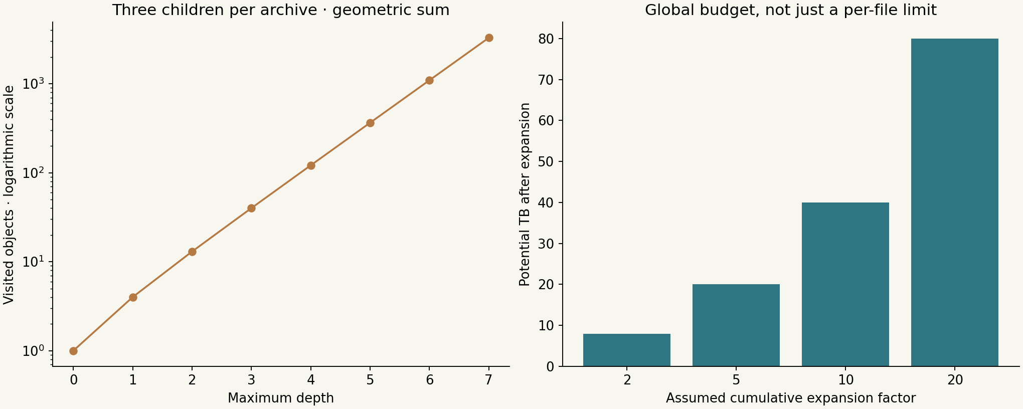
The worker opening archives must not execute discovered files, follow links or write outside the permitted area. Relative names and absolute paths require separate checks before any file is written. Encrypted files, missing volumes, unsupported formats and enormous images need different states. “I could not open it” does not mean “there was nothing to analyze.”
6. A separate network as an analysis environment
The separate environment must allow examination of bytes without executing the intentions they contain. By reassembly in a parallel network, I mean an isolated working laboratory: controlled copies of objects and the relationships needed for analysis. Automatically replaying access attempts, authentication, commands or communications from the observed material would be inappropriate.
The originals remain preserved. Extraction and decoding workers receive identified inputs and return declared outputs. A process converting JPEGs into matrices does not need access to the investigation network, other tools' credentials or the internet. Reducing privileges contains parser failures and makes execution more reproducible.
I would separate queues by cost and operational risk: file identification, archive expansion, decoding, visual derivation and feature extraction. A task is idempotent when repeating it with the same object and configuration does not create contradictory decisions or silently double counts. Its identifier should incorporate configuration; changing analysis resolution creates a different derivation.
result = {status, output_hashes, time, memory, failure_reason}
reprocessing ≠ overwriting previous history
A bounded queue provides backpressure: when decoding cannot keep pace with extraction, intake slows rather than turning all RAM into a buffer. Retries need limits and recorded reasons. A repeatedly failing file must not circulate forever among workers and consume time intended for the rest of the corpus.
7. “It looks like an image” is still a format hypothesis
After checking the header, I would verify that the structure can be traversed, dimensions fit the budget and a compatible decoder produces a valid matrix. An embedded thumbnail does not establish that the main image is complete. A partially readable file may reveal some content while still requiring a truncation flag.
A small compressed image can declare dimensions requiring enormous memory. For 8-bit RGB, the basic matrix occupies approximately W × H × 3 bytes. Converting to 32-bit floating point requires W × H × 3 × 4 bytes, before gradients, pyramids, convolution buffers or library copies.
M_RGB32F = W H × 3 × 4 bytes
4,000 × 3,000 × 3 × 4 = 144,000,000 bytes ≈ 137.3 MiB
Sixteen such images would occupy approximately 2.15 GiB in float32 RGB matrices alone. Temporary allocations can double or triple instantaneous memory. Having 8 GB of RAM does not mean being able to open hundreds of images simultaneously. Concurrency must account for peak memory per worker, not just average JPEG size on disk.
I would record quality and transformations as observation attributes: resolution, orientation, dynamic range, saturation, contrast, blur and missing regions. Analysis transformations might include a reduced-resolution version and a documented color conversion. The preserved file remains accessible through its identifier so decisions can be revisited against the correct source.
Super-resolution and magnification cannot manufacture missing evidence. Interpolation changes the image representation; a generative model may add plausible details that never existed in the record. For this scientific problem, low quality must increase uncertainty and the opportunity to abstain rather than encourage an artificial appearance of certainty.
8. Four terabytes: research time sounded like an HDD
Consider a dimensional calculation with explicit assumptions. I use 4 decimal TB = 4 × 10¹² bytes. TB and TiB are not interchangeable: 4 TiB equals 4 × 2⁴⁰ bytes, roughly 10% more. That small distinction changes hours of reading at this scale.
4 × 10¹² / (80 × 10⁶) = 50,000 s = 13.89 h
This is an idealized sequential-reading bound at 80 MB/s. It excludes mechanical seeks, small files, metadata, copying, decompression and competing processes. The rate is a calculation parameter, not a claimed specification of the drives I received. Sensitivity analysis spans 20–160 MB/s to keep an assumption from becoming a historical benchmark.
Hashing, verified copying, thumbnails and descriptors may require additional passes. A naive design reads and decodes everything for each experiment. A more careful design shares a derivation to avoid repeated work, but adds storage, cataloging and invalidation costs when parameters change.
At an assumed average of 2 MB per image, 4 TB would correspond to two million images. This is not the original corpus count; it illustrates magnitude. A stage consuming two CPU-seconds per image requires four million CPU-seconds. On eight cores at an assumed overall efficiency of 65%, that means approximately 213.7 processing hours.
T_CPU ≈ N × CPU_cost_per_image / (cores × efficiency)
T_CPU ≈ 2,000,000 × 2 / (8 × 0.65) = 213.68 h
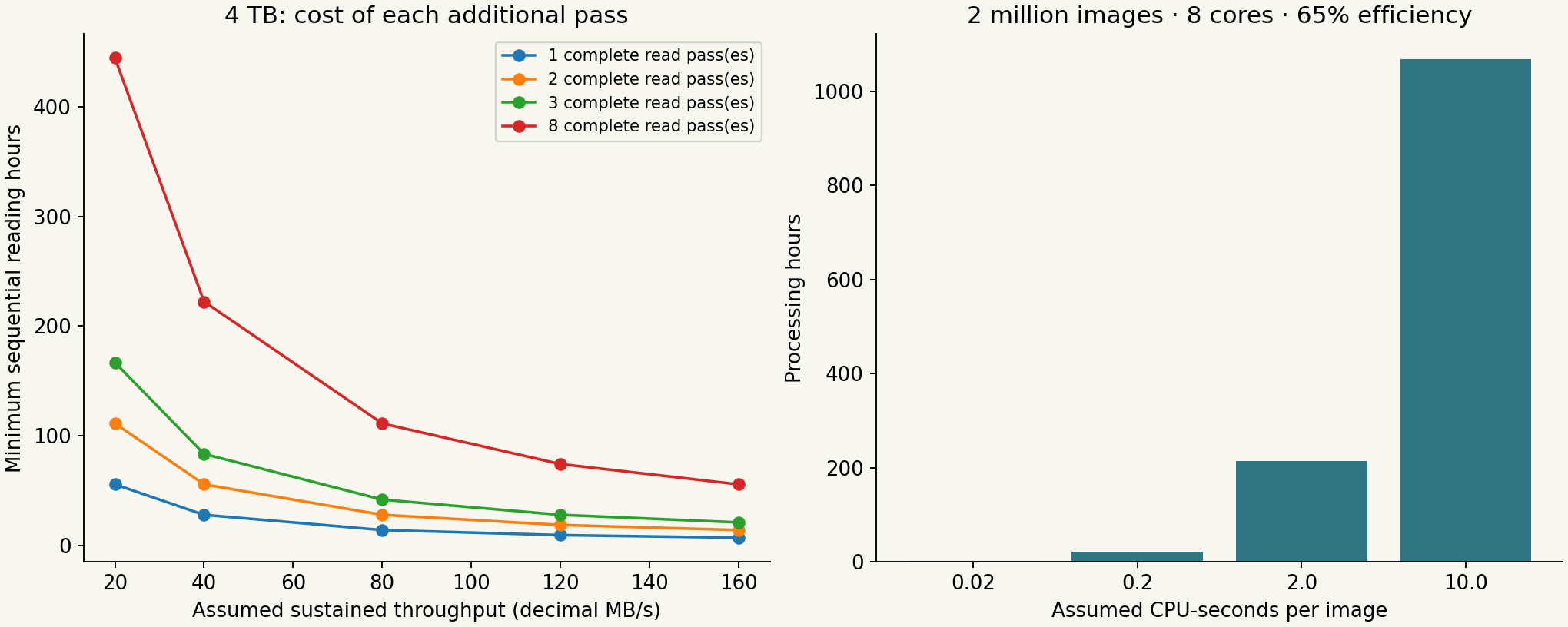
Sustained pipeline throughput is constrained by its slowest stage: if stage capacities are μᵢ, the simplified ceiling is min μᵢ. An individual image's latency includes waiting and successive stages. Confusing throughput with latency leads to promises that eight cores make everything eight times faster, immediately contradicted by disks and serial work.
Amdahl's law makes this limit visible. With serial fraction s and perfectly parallelizable remaining work, speedup on p cores is 1/[s + (1−s)/p]. At s = 0.25, the asymptotic limit is four, however many cores are added. Shared decompression, synchronized catalogs and I/O can increase the portion that does not scale.
Implementation must also control nested parallelism. Eight processes each requesting eight numerical-library threads can produce 64 threads competing for eight cores. Cache, memory bandwidth and context switches consume the expected gain. Experiments should record process and thread concurrency alongside the CPU model.
9. Fitting an image into a representation
A photograph contains an intensity matrix, not ready-made concepts. A descriptor chooses which variations to preserve and which to suppress. If the representation removes relevant information, a downstream classifier cannot recover it. If it preserves too much, it may memorize a camera, border, folder name or background instead of the intended pattern.
Global descriptors summarize whole images or large regions: color histograms, texture and edge distributions. They are relatively compact but may ignore spatial organization. Local descriptors describe regions or interest points; they support correspondences and crops but increase vector counts and search costs.
gradient: gₓ = ∂I/∂x, gᵧ = ∂I/∂y
m = √(gₓ² + gᵧ²), θ = atan2(gᵧ,gₓ)
h_b = Σ_p m(p) × bin_b_weight(θ(p))
A histogram describes a distribution; it does not independently recover a scene. Two images can have similar color histograms and very different content. A crop can remove the context necessary for interpretation. Lighting, compression, pose, distance and resolution change measured features even when a person recognizes relationships between scenes.
Dalal and Triggs's 2005 HOG uses local gradient-orientation distributions with block normalization. It is an important reference for human-shape detection, not a method that independently detects exploitation, nudity, age group or identity. Its usefulness depends on evaluating the representation and classifier for the intended task. [10]
local normalization reduces contrast dependence;
it does not establish invariance to every pose or contextual change
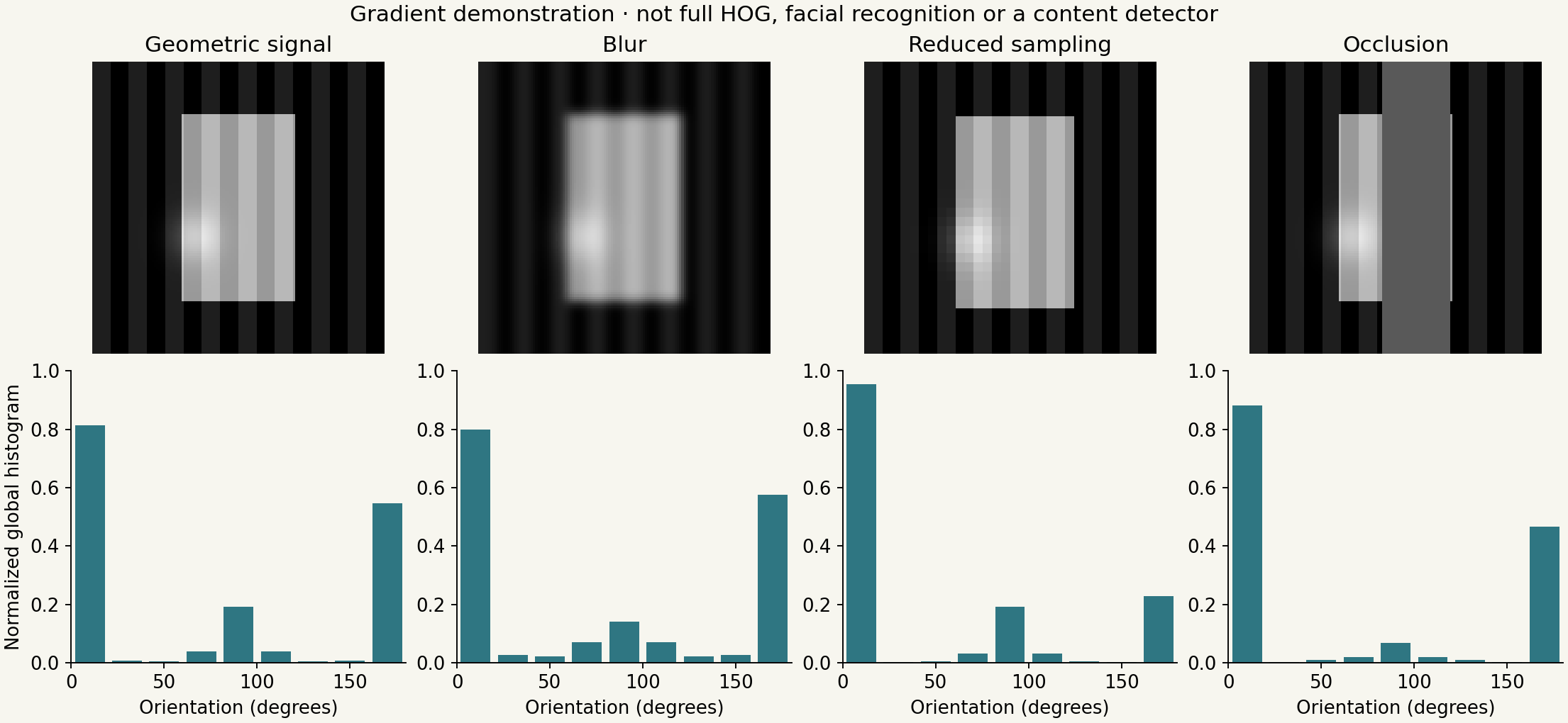
Lowe's SIFT, in its 2004 reference paper, finds scale-space points and describes neighborhoods through gradient orientations. The common descriptor has 128 components. Robustness to certain transformations does not imply semantic equivalence: local matches can arise from repeated textures or backgrounds. Geometric verification checks observational consistency, not truth about people. [11]
SURF, introduced in 2006, combines a Hessian-based detector with approximations and integral images to reduce cost. Efficiency mattered when each extraction second multiplied across millions of files. The relevant comparison would be triage quality per unit of processing, not merely how many points were extracted. [12]
ORB, from 2011, belongs to the continuation of this research period, using binary descriptors and efficiency-oriented choices. Hamming distance counts differing bits in a binary descriptor; indiscriminately using Euclidean distance intended for a different vector changes what comparison means. I do not attribute ORB to a November 2010 implementation. [13]
The descriptors could consume a terabyte too
If each image produced a thousand descriptors with 128 float32 components, that would be 512,000 bytes per image. For two million images, the numbers alone would occupy 1.024 decimal TB. Coordinates, scales, indexes, identifiers and auxiliary structures would still be missing. Reducing pixels to descriptors does not automatically produce a small database.
2,000,000 × 1,000 × 128 × 4 = 1.024 × 10¹² bytes
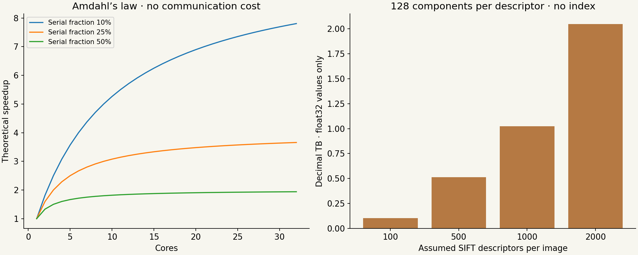
I would need to choose between storing every vector, aggregating descriptors, reducing dimensionality and recomputing some work. This changes memory, query time and traceability. An approximate index may accelerate nearest-neighbor search, but must preserve object retrieval and allow measurement of relevant candidates lost through approximation.
10. Distance, normalization and what the number compares
A color vector, texture vector and gradient histogram do not naturally share units. Adding unscaled components can let the numerically largest feature dominate the comparison. Normalization must be fitted on training data and applied without consulting the test set.
d₂(x,y) = √Σ_j (x_j − y_j)²
d_M(x,y) = √[(x−y)ᵀ Σ⁻¹ (x−y)]
d_χ²(h,g) = ½ Σ_j (h_j − g_j)² / (h_j + g_j + ε)
Mahalanobis distance weights geometry using estimated covariance, but a nearly singular matrix needs regularization and may be poorly estimated with many dimensions and few independent examples. Chi-square distance is an option for nonnegative histograms. Neither can be called a “certainty percentage” without an additional definition and validation.
PCA can project vectors into a subspace: center the data, estimate a basis and retain components. Preserved variance does not mean preserved discriminative information. The most variable background in the corpus may dominate principal components while a relevant class detail accounts for little variance.
Σ U = U Λ; reduced representation z = U_kᵀ(x−μ)
Similarity search can support deduplication or review grouping. Three relationships must remain distinct: exact byte equality, visual similarity between files and a person's identity. An exact hash addresses bytes; a descriptor addresses a visual representation; identity requires another problem formulation, protocol and appropriate evidence. Renaming a column does not cross those boundaries.
11. Training a classifier did not mean writing a rule for every photograph
Manually choosing edges and textures does not mean every decision was a fixed rule I wrote. It was possible to design a representation and learn a statistical boundary. I needed to define each stage's target—for example, prioritizing items for specialist review. A training class is a documented operational convention, not the entirety of a legal or human phenomenon.
A linear SVM computes f(x) = wᵀx + b. Learning adjusts w and b; the descriptor does not provide a ready-made hyperplane. In the soft-margin formulation, C controls the tradeoff between margin and violations. Kernels can express nonlinear boundaries, but bring additional training and prediction costs. [14]
subject to y_i(wᵀx_i+b) ≥ 1−ξ_i; ξ_i ≥ 0
f_kernel(x) = Σ_i α_i y_i K(x_i,x) + b
A dense kernel matrix for two million examples has four trillion entries. In float64, a single matrix would require 32 TB before the rest of training. This is a scaling calculation, not a claim that every solver stores the entire matrix: decomposition, sampling, linear methods and problem organization mattered precisely for that reason.
Random forests, with a 2001 reference, offered an alternative using ensembles of trees and feature sampling. They were another candidate for heterogeneous attributes, with their own cost, memory and generalization assessments. Neither tree votes nor SVM margins should be presumed calibrated probabilities. [15]
I would compare a compact representation and simple classifier before increasing complexity. A more expressive model can memorize leakage faster. If images from one source appear on both sides of an evaluation, better scores may reflect recognition of corpus organization rather than a useful rule for new cases.
12. A dataset begins with human decisions
The annotation unit should not be a folder presumed homogeneous. Each item receives a decision, its provenance, the instruction version and review status. Different categories answer different questions: whether a file is decodable, its visual content, whether review is needed and whether context is available. An incomplete image does not automatically receive a negative label. Insufficiently documented items remain indeterminate.
A useful protocol records disagreements and allows a second reading. Raw agreement can look excellent when almost everything belongs to the majority class. The coefficient κ = (pₒ − pₑ)/(1 − pₑ) discounts agreement expected from label frequencies, but also depends on those frequencies. Neither measure turns consensus into legal truth. The goal is to make the process auditable and discover ambiguities in the instructions.
Training, validation and test splits must be grouped by source or case after controlling duplicates and derivations. Crops, thumbnails and recompressions of the same file must not cross partitions. Tuning a threshold on the test set and reporting that same set as the final evaluation creates optimistic estimates. The test set remains reserved until the procedure is defined; subsequent changes require another independent evaluation.
Protection includes minimal access, access logs and separation of operational identifiers from descriptive data. I publish neither corpus samples nor details that could expose cases. Human work also has costs: breaks, rotation, support and exposure limits are part of review capacity.
13. Content, age, identity and conclusions are different questions
A skin detector is not a nudity detector; a nudity detector does not establish exploitation; a visual classification does not prove age; and image similarity does not identify a person. Backgrounds, lighting, compression, framing and similarly colored materials can produce false positives. Conflating these stages turns a statistical hypothesis into a claim the data cannot support.
Appearance does not establish an exact age, particularly near a legal boundary. Nor does it justify inferring that someone is underage from size, pose or resolution. Sending an item for analysis is a prioritization decision, subject to qualified evaluation and available context. Inconclusive material must retain its uncertainty in the report.
In my record, engineering should narrow the search without replacing human responsibility. That requires abstention categories and traceable referral reasons. A terse output such as “positive” discards essential information: input quality, model version, validation population, threshold and reason for review.
14. CNNs: learned representations and an operation budget
Convolutional networks already had an established foundation before this period, including LeNet [16]. A convolution computes yᵢⱼₖ = bₖ + Σᵤᵥ꜀ wᵤᵥ꜀ₖ xᵢ₊ᵤ,ⱼ₊ᵥ,꜀. Weight sharing reduces parameters compared with a dense connection across every pixel. However, each spatial position still requires operations. Pooling reduces resolution and changes sensitivity to small displacements; it does not guarantee invariance to every transformation.
For stride-one convolution without padding, Hₒ = Hᵢ − K + 1, and the multiply–accumulate count is HₒWₒCₒK²Cᵢ. An illustrative grayscale network with six 5×5 filters, 2×2 pooling and then sixteen 5×5 filters requires 357,600 MACs for a 32×32 input and 10,380,000 for 128×128, counting only forward convolutions. Training adds gradients, activation storage and parameter updates. A MAC is not a unit of CPU time.
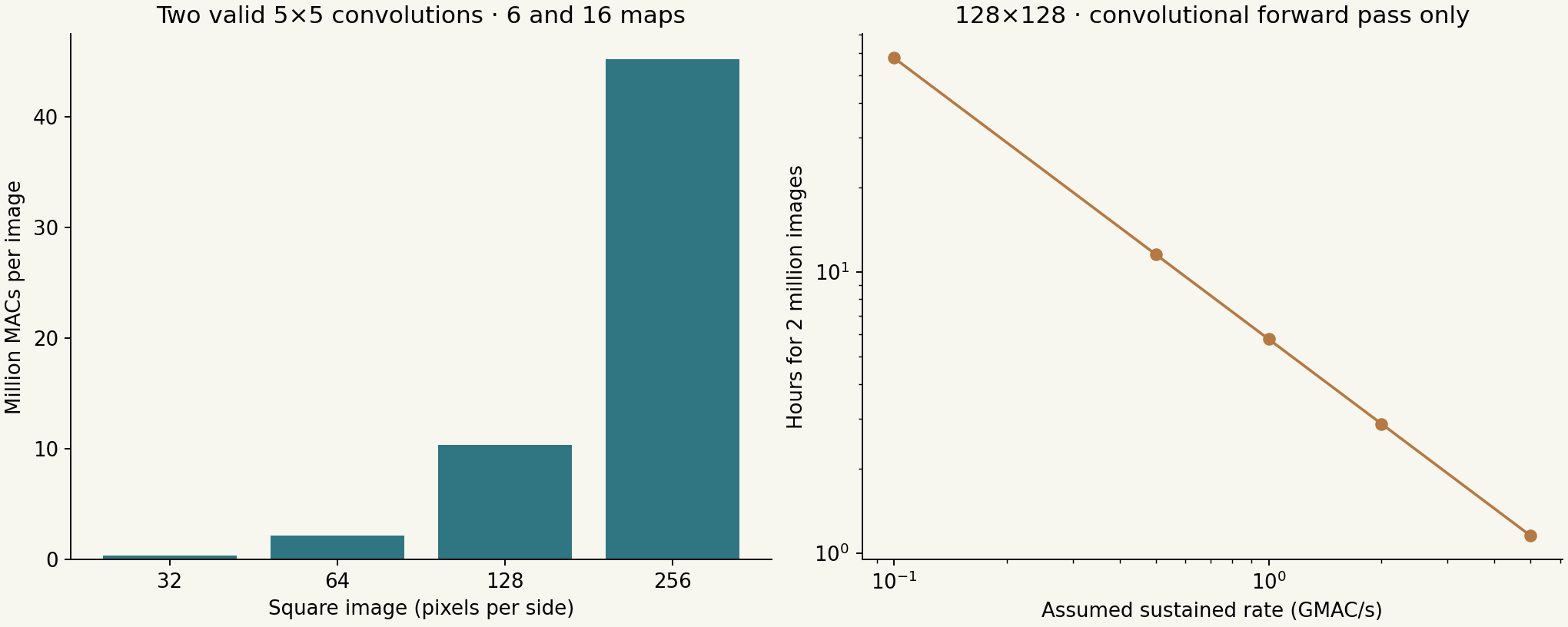
A loss such as cross-entropy guides learning; it does not independently solve annotation quality or distribution shift between sources. A small network could be an experimental alternative alongside traditional descriptors and classifiers. GPU research in 2011 already demonstrated the importance of parallel implementation [5]. It would be wrong to say GPUs or CNNs did not exist; practical limits involved data, tools, infrastructure and engineering time.
15. Margins, probabilities and abstention
An SVM output is a margin, not a probability. The sigmoid transformation P(y=1|f) = 1/(1 + exp(Af+B)), associated with Platt's method and the implementation discussed by Lin and colleagues [17], learns A and B using separate data. Calibration requires representative samples without source leakage. Returning 0.9 does not automatically mean 90% accuracy for every population.
The Brier score, the mean of (pᵢ−yᵢ)², evaluates probabilistic predictions; reliability diagrams compare observed frequencies with average predictions. Too few bins hide detail; too many become unstable. An attractive curve may result from a small sample, duplicates or a distribution unlike the next input.
Two thresholds can distinguish low-priority, review and priority-review regions. This does not mean automatically clearing files below a value. Decoding failures, unknown formats and low quality follow an exception path. Thresholds depend on purpose, error costs, review capacity and authorized evaluation. The following values are exclusively mathematical demonstrations.
16. When 95% sensitivity still produces a poor queue
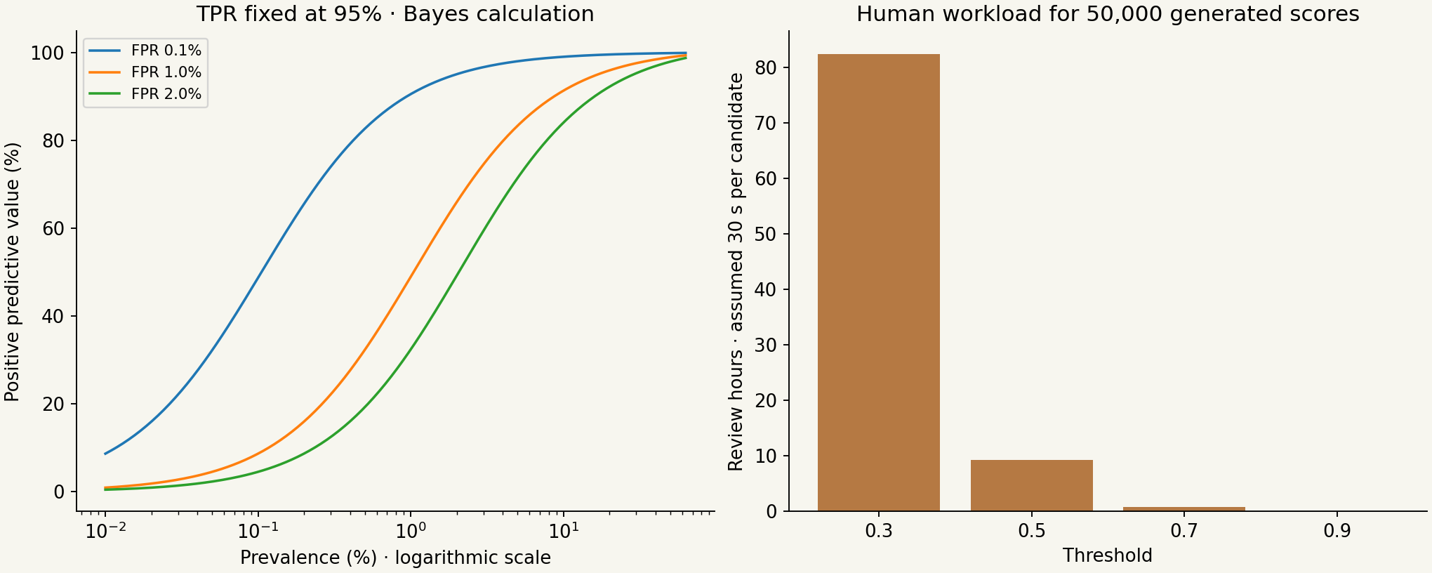
Sensitivity is TP/(TP+FN), false-positive rate is FP/(FP+TN), and precision is TP/(TP+FP). Precision depends on prevalence π: PPV = TPR·π / [TPR·π + FPR·(1−π)]. At π = 0.001, TPR = 0.95 and FPR = 0.02, expected precision is approximately 4.54%. Most referrals would be false even though sensitivity alone looks high.
To visualize this effect without sensitive images, the supplement generates 50,000 numerical scores: 250 analytical positives and 49,750 negatives. These are beta-distribution samples using seed 2010, with no training or images. The experiment does not evaluate the historical work, a forensic tool or the prevalence of any corpus.
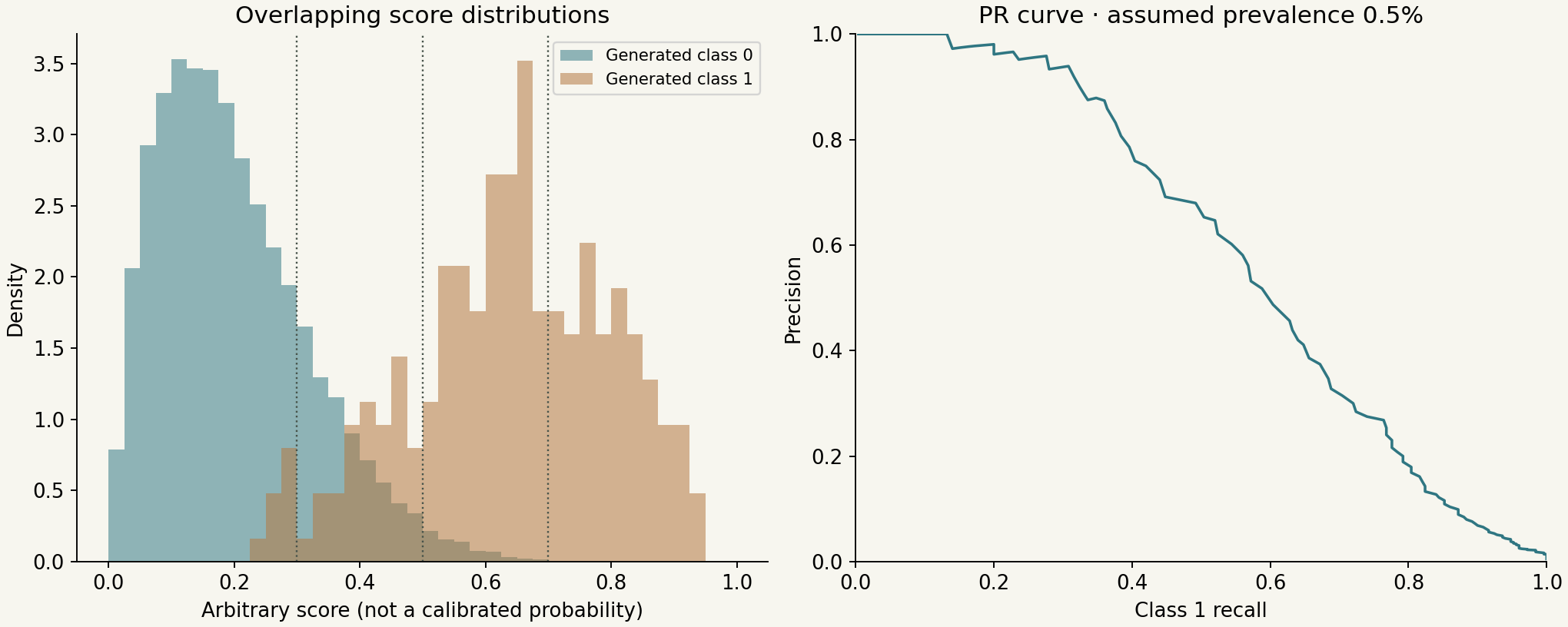
| Threshold | TP | FP | FN | Precision | Queue |
|---|---|---|---|---|---|
| 0.3 | 241 | 9,653 | 9 | 2.44% | 9,894 |
| 0.5 | 201 | 920 | 49 | 17.93% | 1,121 |
| 0.7 | 90 | 13 | 160 | 87.38% | 103 |
| 0.9 | 9 | 0 | 241 | 100% in this sample | 9 |
The last result does not prove the absence of false positives in the population. It coincides with missing 241 of the 250 generated positives. Reporting only “100% precision” would conceal the main cost. Uncertainty intervals, denominators and test composition must accompany evaluation.
17. Human review is a finite resource
At thirty seconds per item, the 9,894 referrals in the first row require 82.45 hours of uninterrupted review; 1,121 require 9.34 hours. This excludes breaks, second readings and contextual research. Arrival rate λ must be compared with effective service capacity μ. When λ remains above μ, the queue grows regardless of descriptor-extraction speed.
I therefore need to observe queue length, item age, rejected formats and review by source. Distribution shift can increase the queue without an explicit software failure. Updating a model or changing a threshold requires preserving the previous version and recording changes. An auditable evaluation does not erase earlier decisions to present only the most favorable configuration.
18. Personal record: 2012 and 2022
These four photographs are mine, supplied and identified by me. The two with a dress shirt/polo shirt date from 2012; the two with tank tops date from 2022. They form a personal record later than the 2010–2011 study period. They are not corpus samples and were not used in this article's calculations.



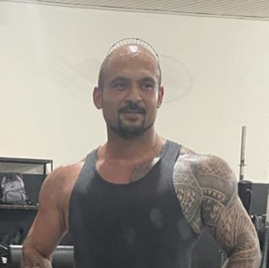
Lighting, clothing, framing and the passage of time illustrate why visual comparison needs context. I present no facial recognition, age estimation or biometric percentage for these photographs. Attribution and dates are my statements. Distance between vectors can measure a representation; a simple rescaling cannot turn it into the probability that two people are the same person.
19. A verifiable procedure without disclosing the confidential implementation
- Record authorized scope, receipt, integrity and responsible parties.
- Work on copies and maintain a verifiable link to the source.
- Extract objects from available streams, recording gaps and limitations.
- Inventory archives and enforce depth, volume and time budgets.
- Decode in isolation and distinguish failures from negative results.
- Measure quality and produce descriptors with versioned configurations.
- Evaluate models using source-grouped partitions and a reserved test set.
- Record scores, applicable calibration, thresholds and exception paths.
- Refer items for qualified review while preserving disagreements.
- Report evidence, decisions and limits without turning priority into a conclusion.
for each authorized_object:
    record_source_and_integrity(authorized_object)
    result = extract_with_budget(authorized_object)
    if result.incomplete:
        record_exception(result)
        continue
    image = decode_in_isolation(result)
    if image.failed:
        record_exception(image)
        continue
    record_quality_and_versions(image)
    route_under_review_protocol(image)
This pseudocode describes responsibilities, not the complete implemented solution. Keys, cases, confidential rules, internal configurations and patents remain protected. No part enables access to third-party networks or collections.
20. What came later—a separate timeline
AlexNet, from 2012 [18], made the combination of convolutional networks, data and GPUs particularly visible in classification. ResNet appeared as a preprint in 2015 and a conference publication in 2016 [19]. Vision Transformer emerged in 2020, with publication in 2021 [20]; CLIP dates from 2021 [21]. I do not attribute these technologies to the November 2010 work.
Later representations expand transfer and retrieval possibilities, but require task-specific evaluation. NIST's age-estimation evaluation, published in 2024 [22], belongs to this later commentary: image quality and test population remain relevant. It does not retrospectively validate a 2010 system or turn appearance into proof of age.
21. An analytical supplement to run at home
The package contains Python, tables and instructions for regenerating all seven figures. It uses equations, numerical distributions and a geometric signal. It contains no personal photographs, corpus images, network capture, facial recognition or content detector. The listed library versions describe the supplement's current execution environment; they are not attributed to the 2010 environment.
Download Python, figures and tables ↓
python3 -m venv .venv
source .venv/bin/activate
python -m pip install -r requirements.txt
python figures.py
python verify.py
Assumptions are editable: reading throughput, estimated image count, CPU cost, parallel efficiency and review time. Changing them produces a different capacity scenario, not a measurement of the historical case.
22. Conclusion: narrow the search and preserve uncertainty
The problem I remember was not merely choosing a classifier. Four terabytes meant reading, copying, archives, decoding, descriptors, memory, queues and people. A local improvement could shift the bottleneck downstream. An apparently high metric could create an impractical queue or conceal false negatives.
The scientific value lies in stating units, separating assumptions from measurements and preserving the provenance of every decision. This article is part of a personal historical record. I present techniques available or developed for that problem without fully disclosing their implementation. People, companies, confidential information and patents remain protected and belong to their respective holders, as do my own patents.
References and credits
- Falcão — Image Foresting Transform, author’s bibliography ↗
- OpenCV — release history ↗
- LIBSVM — historical releases ↗
- OpenMP 3.0 — specification, 2008 ↗
- Cireșan et al. — Flexible, High Performance Convolutional Neural Networks, 2011 ↗
- NIST SP 800-86 — Guide to Integrating Forensic Techniques into Incident Response, 2006 ↗
- RFC 793 — Transmission Control Protocol, 1981 ↗
- RFC 1952 — GZIP file format, 1996 ↗
- Library of Congress — 7z format description ↗
- Dalal and Triggs — Histograms of Oriented Gradients, 2005 ↗
- Lowe — Distinctive Image Features from Scale-Invariant Keypoints, 2004 ↗
- Bay, Tuytelaars e Van Gool — SURF, 2006 ↗
- Rublee et al. — ORB, 2011 ↗
- Cortes and Vapnik — Support-Vector Networks, 1995 ↗
- Breiman — Random Forests, 2001 ↗
- LeCun et al. — Gradient-Based Learning Applied to Document Recognition, 1998 ↗
- Lin, Lin and Weng — A Note on Platt’s Probabilistic Outputs for Support Vector Machines ↗
- Krizhevsky et al. — ImageNet Classification with Deep Convolutional Neural Networks, 2012 ↗
- He et al. — Deep Residual Learning, 2015/2016 ↗
- Dosovitskiy et al. — An Image Is Worth 16×16 Words, 2020/2021 ↗
- Radford et al. — Learning Transferable Visual Models, 2021 ↗
- NIST IR 8525 — Face Analysis Technology Evaluation: Age Estimation and Verification, 2024 ↗
Personal photographs: Klyff Harlley Toledo; dates and authorship supplied by the author. The account of receiving material from Brazil’s Federal Police is the author’s historical statement; this article does not disclose case data or confidential documents.